How many agents should you run?
Running a fleet of agents spends two currencies at once: wall-clock time and tokens. More agents in parallel finish sooner but burn more tokens; fewer agents are cheaper but slower. Where you should sit on that trade depends on the price you put on latency versus compute — and, more than anything, on the shape of the problem. Two toy models bracket the cases we care about: blind search, and a climb up a foggy mountain. They give opposite answers, and the gap between them is the whole design question.
Fix a task and let \(N\) the agents loose. Two numbers summarize a run: the expected time to finish, \(\langle T\rangle\), and the expected token spend, \(\langle C\rangle\). Because every agent that is alive in a round consumes tokens that round, token cost is just agent-count times time, \(\langle C\rangle = N\,\langle T\rangle\). Choosing \(N\) is choosing a point on a time–token frontier. To pick one point we need a price. Write the total cost of a run as a weighted blend
\[ \text{Cost} \;=\; a\,\langle T\rangle \;+\; b\,\langle C\rangle, \]
where \(a\) is what you pay for latency (the value of finishing one unit of time sooner) and \(b\) is the price of a token. The ratio \(a/b\) is the only thing that matters: it says how many tokens you would happily spend to save one unit of time. A line of constant Cost in the time–token plane is an iso-cost line, and the best \(N\) is where that line is tangent to the frontier.
Take the simplest model of looking for a needle: \(N\) independent, memoryless agents. Each round, each agent independently finds the answer with probability \(p\). At least one of them succeeds in a given round with probability \(p_N = 1-(1-p)^N\), and the number of rounds to first success is geometric, so
\[ \langle T\rangle \;=\; \frac{1}{1-(1-p)^N}, \qquad \langle C\rangle \;=\; N\,\langle T\rangle \;=\; \frac{N}{1-(1-p)^N}. \]
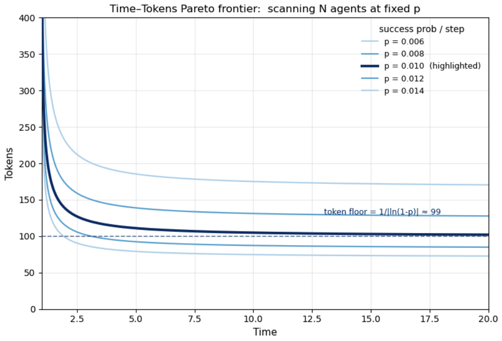
The token floor. What happens for small \(N\)? Write \(1-(1-p)^N = 1-e^{N\ln(1-p)} \approx N\,\lvert\ln(1-p)\rvert\) when \(N\) is small. The agent factor cancels:
\[ \langle C\rangle \;=\; \frac{N}{1-(1-p)^N} \;\xrightarrow[\;N\to 0\;]{}\; \frac{1}{\lvert\ln(1-p)\rvert} \;\approx\; \frac{1}{p}. \]
So the cheapest possible way to solve the problem costs about \(1/\lvert\ln(1-p)\rvert\) tokens, achieved by running essentially one agent and waiting. The remarkable part is how flat the rest of the frontier is. Eliminating \(N\) in favor of the time \(T\) gives the frontier in closed form,
\[ \langle C\rangle(T) \;=\; \frac{T}{\lvert\ln(1-p)\rvert}\,\ln\!\frac{T}{T-1}, \]
which falls to the floor \(1/\lvert\ln(1-p)\rvert\) as \(T\) grows and rises only logarithmically as you drive \(T\) toward its minimum of one round. In speedup terms, \(S(N) = \langle T(1)\rangle/\langle T(N)\rangle = \big(1-(1-p)^N\big)/p\): near-linear for small fleets (\(S\approx N\) while \(Np\ll 1\)) and saturating at a hard ceiling of \(1/p\). Breadth is embarrassingly parallel right up to that ceiling, and buying speed costs almost no extra tokens.
Minimize \(\text{Cost}(N) = (a + bN)/\big(1-(1-p)^N\big)\) over \(N\). Writing \(L \equiv \lvert\ln(1-p)\rvert\) so that \((1-p)^N = e^{-LN}\), the first-order condition is \(b\big(1-e^{-LN}\big) = (a+bN)\,L\,e^{-LN}\). The clean way to read it is to substitute \(u \equiv LN\), which eliminates \(N\) and leaves a single transcendental equation for the unknown \(u\):
\[ e^{u} - u - 1 \;=\; \frac{aL}{b} \;\approx\; \frac{ap}{b}, \qquad\text{then}\qquad N^\star = \frac{u^\star}{L}. \]
The root \(u^\star\) has an exact closed form: with \(r \equiv aL/b\) and \(c \equiv 1+r\), it sits on the \(W_{-1}\) branch of the Lambert \(W\) function,
\[ u^\star \;=\; -\,c \;-\; W_{-1}\!\big(-e^{-c}\big), \qquad N^\star = \frac{u^\star}{\lvert\ln(1-p)\rvert}. \]
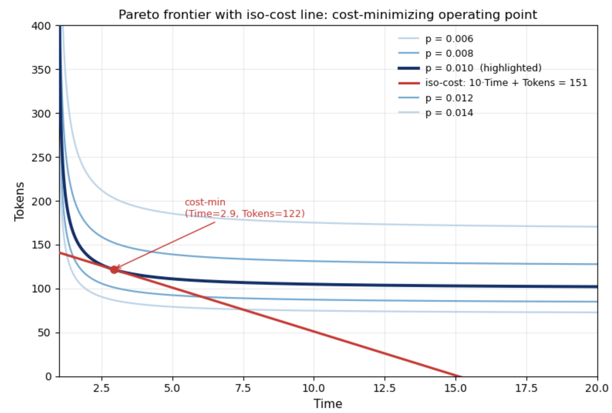
For large \(r\), \(e^{u^\star}\approx r\), so \(u^\star \approx \ln(aL/b)\) and \(N^\star \approx \ln(aL/b)/L \approx \ln(ap/b)/p\): the cost-minimizing fleet grows only logarithmically in how much you value speed. Even when latency is precious, a search problem rewards only a modest crowd of agents.
Now the opposite regime — and the one that fits most real agentic work. A great many programming and research tasks share three features. First, there is a measurable notion of progress toward a goal: the fraction of unit tests passing, a benchmark score, a shrinking loss curve, the number of lemmas left in a proof, a backtest's Sharpe. You cannot see the summit, but you can always tell roughly how high you currently are. Second, the ease of further progress depends on how far you have already come: the first 80% of a feature is usually far cheaper than the last 20%, an early refactor opens easy wins while the final edge cases grind, and a noisy backtest gets harder to improve as the obvious signal is used up. Third, when several attempts are in flight, a sensible policy is to build on whichever attempt has gotten furthest — keep the best partial solution and try to extend it, rather than averaging the attempts or restarting from scratch.
The foggy mountain is the minimal model with exactly those three properties, and each maps to one ingredient. Progress is a scalar \(h\in[0,1]\) we can measure (property 1). The rate at which proposals improve on the current best is set by \(\lambda(h)\), which may depend on the height already reached (property 2). And every round, all agents restart from the best \(h\) found so far and we keep the best new proposal (property 3). The “fog” is that no agent can see the path ahead: it can only propose a local step and learn the step's value by taking it — exactly as an agent only learns whether an edit helps by running the tests or the backtest. This pooling onto the current leader is what makes it a depth problem: unlike blind search, the agents are not independent tries at the answer but competing draws for the single best next step.
Concretely: \(N\) agents climb in fog; progress \(h\in[0,1]\) starts at \(0\), and reaching \(h\ge 1\) is success. Each round, all agents start from the best height so far, each proposes an improvement, and we keep the best. We take a single agent's proposed gain above the current best to be exponential — the maximum-entropy choice given only a mean step size, and memoryless, so no agent has private information about where the next improvement lies:
\[ p\big(h^{(i)}\mid h_t\big) \;=\; \lambda\, e^{-\lambda\,(h^{(i)} - h_t)}, \qquad h^{(i)} \ge h_t. \]
The round's progress is the best of \(N\) independent exponentials, and the expectation of that maximum is the classic harmonic result \(\mathbb{E}[\max] = H_N/\lambda\), where \(H_N = \sum_{k=1}^{N} 1/k\). Advancing \(H_N/\lambda\) per round, the climb to \(h=1\) takes
\[ \langle T\rangle \;=\; \frac{\lambda}{H_N}, \qquad \langle C\rangle \;=\; N\,\langle T\rangle \;=\; \frac{N\lambda}{H_N}. \]
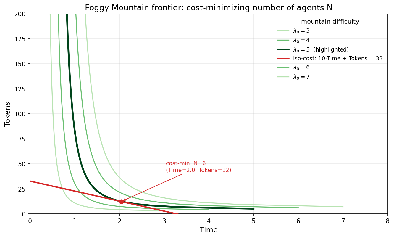
Robust to terrain. The uniform-\(\lambda\) assumption is not essential. If difficulty varies with height, \(\lambda = \lambda(h)\), then per round \(dh/d(\text{round}) = H_N/\lambda(h)\), and integrating from \(0\) to \(1\) gives \(\langle T\rangle = \bar\lambda/H_N\) with \(\bar\lambda = \int_0^1 \lambda(h)\,dh\) the mean difficulty. The same laws hold; only the average steepness enters.
The speedup is logarithmic. Here \(S(N) = \langle T(1)\rangle/\langle T(N)\rangle = H_N \approx \ln N + \gamma\). There is no ceiling — but there is no leverage either. Doubling the fleet adds a flat \(\ln 2 \approx 0.69\) to the speedup, forever. To halve the time you must roughly square the number of agents. Minimizing \(\text{Cost}(N) = \lambda(a+bN)/H_N\) gives the optimum \(N^\star\,(H_{N^\star}-1) = a/b\), i.e. \(N^\star \approx (a/b)/\ln N^\star\) — nearly linear in the price ratio, where search was only logarithmic.
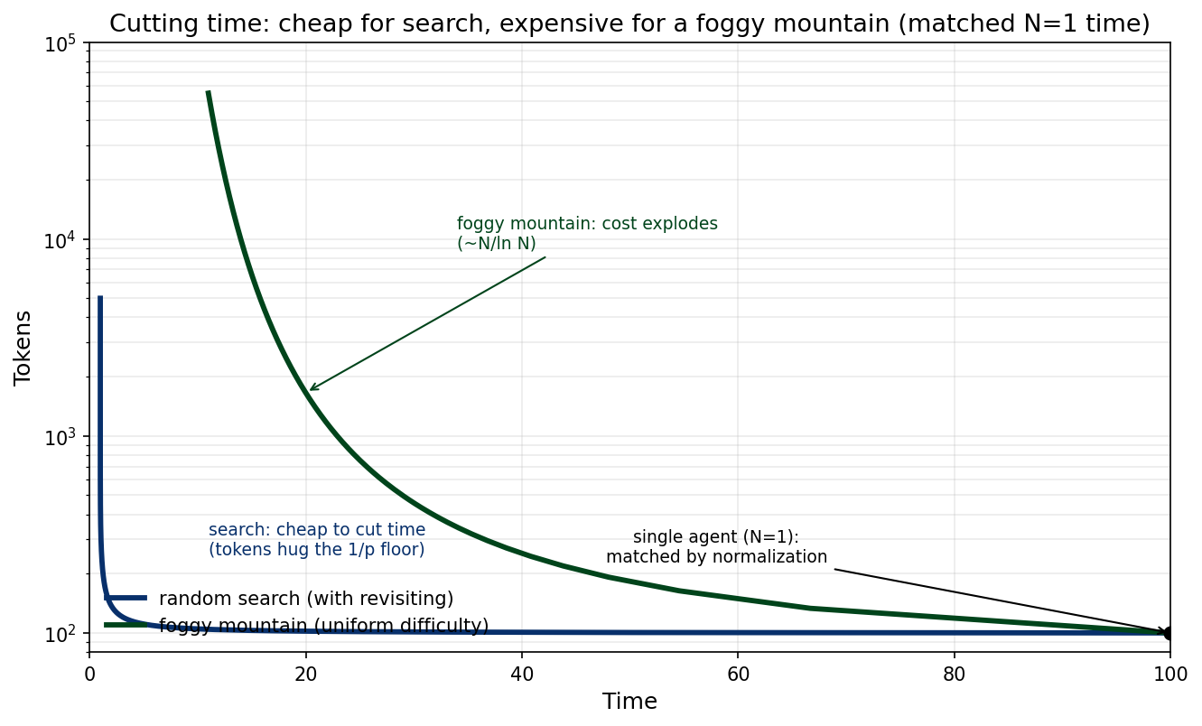
Side by side the two regimes invert each other on every axis:
| Quantity | Search (breadth) | Foggy mountain (depth) |
|---|---|---|
| Time \(\langle T\rangle\) | \(1/\big(1-(1-p)^N\big)\) | \(\lambda/H_N\) |
| Speedup \(S(N)\) | \((1-(1-p)^N)/p \to 1/p\) | \(H_N \approx \ln N\) |
| Token floor | \(1/\lvert\ln(1-p)\rvert\) | none — cost \(\sim N/\ln N\) |
| Optimal fleet \(N^\star\) | \(\sim \ln(ap/b)\,/\,p\) | \(\sim (a/b)/\ln N\) |
The same iso-cost machinery, two opposite verdicts. Breadth saturates and stays cheap; depth never saturates but makes you pay nearly linearly for every increment of speed.
The intuition is simple. In search, any one agent can solve the whole problem, so a second agent is a fresh independent lottery ticket — until the per-round success probability nears one and further tickets are wasted. On the mountain, agents are not independent tries at the answer; they are competing draws for the single best next step, and the expected best of \(N\) draws from a tail grows only like \(\ln N\). Redundancy is the price of depth.
Agentic research for markets is part breadth and part depth, and the two halves want opposite fleet sizes. Scanning a wide hypothesis space — which features, which instruments, which regimes — is search: cheap to parallelize, so fan out wide and let the \(1/p\) floor work for you. Refining one strategy through a noisy, non-stationary backtest is a foggy-mountain climb: each iteration is a small expected step up a tail, the speedup is logarithmic, and a bigger crowd mostly buys redundant proposals. That asymmetry is exactly why our evolutionary loops lean on structure — islands, migration, quality-diversity selection — rather than brute parallelism: structure converts a depth problem back into a breadth problem by keeping many semi-independent climbs alive at once. The math here is the budgeting layer beneath that design, and it connects directly to the noisy-rewards work.